|
Performance and strength metrics in EliseMeasuring performance and controlling for luck-based factors in computer Scrabble® play Although Elise is an extremely strong Scrabble® player, I am still interested in improving its play further. The simplest way to improve Elise's play strength is to improve the play of its static move evaluator -- that is, to improve the move-evaluation algorithms used by Elise's 'quick move'. It is easy to test changes in this code, and determine exactly how much improvement (if any) they make in Elise's 'quick move' play. This is because you can play many thousands of 'quick move' games in minutes, and if the new changes make any difference in the quality of play it will become apparent quickly. But there are other, trickier ways to improve Elise's strength -- changes in the simulation code, for example, or clock management changes, or improvements in Elise's tile inferences. These sorts of changes are not easily tested in the same way, since they require many simulation games to be played, and each game might take 20 or 30 minutes to complete. I expect that Elise is quickly approaching the point in which significant boosts in strength will come primarily through improvements such as these, that are much harder to test than changes in its static evaluation. With the newest version of Elise (0.1.8), there is now the ability to run strength tests on your computer. These tests will play games of Scrabble® using experimental new features in Elise's move evaluation and tile inference code. The results are sent back to this website (the GCG files are copied into this folder for all to see and enjoy.) This feature allows me to split the testing work among many computers, and get a lot of simulation games quicker. These tests will allow me to determine which of these features improve play strength, and about by how much. Just as importantly, this data can help me to measure the trade-off between better evaluations and more time spent in the move evaluation code. Some changes might improve the quality of move evaluation significantly, but at the same time reduce the performance of the evaluator to the point where the feature loses to simply increasing the simulation ply. (We can always boost strength by increasing simulation ply, and if that performs better than the experimental features, then the new feature doesn't actually help.) But there are many random factors in Scrabble®, and in comparing performance of two algorithms it is important to be able to control for these random factors somehow. In a small sample size of games, the random elements of tile draws can dominate any skill differences between two players. Since, in these new tests, the two players are both just Elise with different settings, the difference in play strength is likely to be (relatively) small. I can always wait until I have many thousands of games in order to evaluate the experimental features, of course, but even then there may be too much noise to reliably draw conclusions unless we first have some ways to control for the random elements in Scrabble® play. I actually have developed several such methods, and I'd like to explain them briefly on this page. To illustrate the application of these methods, we'll use a dataset I have available right now: the testing games Elise has played against Quackle at various stages in its development over the past few months. In most of these games, Elise has been set at either fixed 3 ply simulation or a 10-minute clock game (on a several years-old Dell Optiplex 755 with 2 GB RAM, and quadcore Intel Core 2 Q6600 clocked at 2.4 GHz.) There are 302 games total in this dataset. These are all English-language games; 142 are TWL06, 106 are CSW12, and 54 are TWL98. Since both Elise and Quackle have perfect word knowledge and board vision -- neither player will miss any legal move -- we can rule out any disparities in these factors. This is one way in which examining computer v. computer games makes this sort of analysis easier. If we were examining games between human players, we would have both of these factors as possible skill elements that could differ among players, and they would surely be difficult to isolate without many, many games. Among human players, I suspect that differences in word knowledge and board vision are actually larger than other skill-based differences. Among computer players, there is no difference in these factors. You can see the results of these 302 games here. GCG files for most of these games are available in the game collection. There is a measure implemented in Elise, for estimating tile luck, which is computationally expensive. Since it is expensive to calculate, I intend to only use it sparingly in examining the strength test results -- only when it's necessary. This is the "rate current rack draw" feature in Elise, available from the "Rack" menu. This feature quantifies rack draw luck by starting with the player's rack leave from their previous move (or an empty rack at the beginning of the game), filling it with tiles drawn from the pool of unseen tiles, determining the best move on the board, and repeating that thousands of times. By comparing the actual rack draw to the thousands of simulated rack draws, we can get a good estimate of what portion of all possible rack draws are worse (or better) than the actual one. Since this takes some time to evaluate, it's best to only use it when you really need it -- when you can't get a reasonable answer using any of the several simpler methods I'll explain here. It's here if we need it, if the data is "too close to call", but it's not the first tool to take out of the toolbox. There is an extremely simple measure that partially controls for tile luck by adjusting for the most important element of tile luck, blank draws. Simply break the player's record into three categories: their record when holding no blanks, their record when holding only one blank, and their record with both blanks. If a player's record is winning when blanks are even, that player is probably superior to his or her opponents. If a player wins more games with zero blanks than they lose when drawing both blanks, that is also an indication that they are probably a better player than their opposition. Let's try this with the 302 testing games in our example dataset:
Elise's record, with exactly one blank, is almost the same as its overall record, just over 61% winning versus Quackle. (Draws are counted as half a win in the win percentages above.) Elise wins 30% of the games in which it draws no blanks, and loses only 10% of the games in which it draws both blanks -- this is also indicative of a strength difference between the two players. This is a simple way to roughly control for tile luck, but it is only useful if there is a substantial difference between the two players. If the difference in strength is small, you would still need many thousands of games to get a reasonable answer from this very simple method. Going forward, I expect most of the strength differences from experimental features to be quite small, so this method will probably not give a conclusive answer very often. Another metric, also easy to calculate, is to look at the average value of each player's racks. This value can be estimated by using Elise's rack statistics -- for each rack Elise can produce a good estimate of value, relative to the overall average rack. Let's call this metric the "average relative rack value", ARRV.
Example of ARRV calculation The ARRV is mostly random from game to game. Sometimes a player will get both blanks, the Z and X, and three esses, and have an ARRV of 10. Sometimes a player will repeatedly draw six vowels and end up with an ARRV of -8. In most games the ARRV will be somewhere between -3 and 5. Although ARRV is mostly random, there is some skill component involved: most expert players (and all competent computer players) will have an average ARRV, over many games, greater than zero (in fact, for most expert players the long-term average will be somewhere around 2). This is because they take care to give themselves good tile leaves -- they do not turnover good tiles unless they have an excellent play. They are also quick to exchange when their racks are very bad. A poor player might have an average ARRV below 0. An average player will have an average ARRV above zero -- this is because you can have a single-game ARRV, in an exceptional case, of 12 or more, while single-game ARRVs below -9 or so are almost never seen. ARRVs, in other words, can be said to have a distribution with a slightly longer right tail than left tail. No matter how good a player you are, though, over hundreds of games (in English language play) it is impossible to have an ARRV greater than approximately 3 (assuming, of course, you are playing to win and not fishing for better tiles almost every turn, or passing with a fantastic rack). This is because the random component of ARRV is much greater than any skill component. You can't consistently have tile luck that good over hundreds of games (if you're actually playing the game) -- in about 25% of games, you aren't going to get any blanks, and individual racks without blanks with relative values greater than 20 are rare. Blank-less games will often have an ARRV well below zero. On the other side of the scale, if you're an expert player, you are also highly unlikely to have an average ARRV below approximately 1.20 over any large number of games. (Novice players might, by poor rack management, sustain lower averages than this.) (Note: the ARRV ranges I've quoted are based on TWL06 or CSW12 play; the values are similar for both lexicons. It is probable that using other languages or lexicons, the typical ARRV ranges may be larger or smaller than this.) ARRV, by itself, is not a measure of play strength, even over large numbers of games. A player who fishes for tiles too often will have a large average ARRV. A player with poor word knowledge may miss plays with good racks, and have a large average ARRV. An extremely skillful player may get more out of bad or mediocre tiles than other players, and have higher turnover with good tiles by playing lots of bingos, and accordingly have a relatively small average ARRV. And given the primarily-random nature of ARRV from game to game, any smallish differences in average ARRV are more likely to be attributable to chance than any sort of skill. But ARRV, interpreted the right way, can point to a strength difference. Among players of comparable skill, the ARRV gives you information about the result of the game -- given two players of equal skill, the player with the higher ARRV wins the game about 75% of the time. This should not be terribly surprising: given two players of equal ability, you expect the player with the better racks to win most of the time -- but it is a quite strong result, and useful for what I need it to do. Furthermore, the difference in ARRV between the players is positively correlated with the final point spread in the game, and the larger the difference in ARRV, among two opponents of equal skill, the more likely it is that the player with the higher ARRV won the game. To illustrate this relationship, I had Elise play 1,000 games against itself. Both Elise players used the 'hi-leave' algorithms to determine their moves. Since both used the same algorithms to determine their moves, both players were equally strong. This table illustrates how the difference in ARRV corresponds with win probability and point spread:
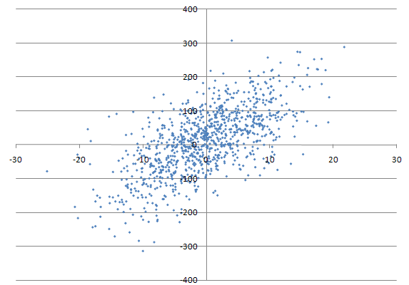
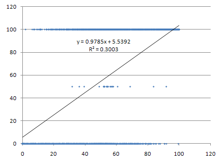
You might notice there is a slight asymmetry here, as player 1 wins about 80% of the games in which it is ahead in ARRV, while player 2 wins about 70% of the games in which it is ahead in ARRV. This is simply because "player 1" is the player who always plays first, and playing first is an advantage in Scrabble®. I thought that I might remove this asymmetry by examining, not the average relative rack value, but rather the total relative rack value, but that does not appear to be a meaningful improvement (possibly because there is also the issue at the other end of the game, the player emptying the bag being at a slight disadvantage.) You can adjust for this by giving the second player an ARRV penalty, to make a difference in ARRV mean the same thing for both players. This is only relevant if you're looking at a very small number of games, or a set of games in which a player plays first many more times than second (or vice versa) -- if you're looking at a set of games in which a player is first player 50% of the time, and second player 50% of the time, it is much less important. In any case, if you know which player has the higher ARRV, and you know the players are about equally strong, you can tell me the winner of the game and be right about three times in four. If you know that one player had a substantial advantage in ARRV, you can be even more confident about the outcome of the game. If we have a set of games of interest that is sufficiently large, then we can compare performance in those games to what we would expect based on differences in ARRV. If one player wins most of the games in which he is at a disadvantage in ARRV, for example, that is strong evidence that this player is stronger than his opposition. Indeed, if we have a large number of one player's games, and he wins only 35% or 40% of the games in which he is behind in ARRV, that is still evidence that he is stronger than his opponents -- we would expect that player to only win only about 25% of the games in which he had a smaller ARRV than his opponents. Where the performance deviates significantly from the expectations based on ARRV, assuming our sample is large enough, we can attribute much of that difference to skill -- or at least, factors other than tile luck. In version 0.1.8, Elise will show you ARRV for each player from the "Game statistics" option in the "Game" menu. Can we apply ARRV to our Elise v. Quackle dataset? Sure we can. In that set, there are 157 games in which Elise had a lower ARRV than Quackle. In those 157 games, Elise played first 82 times and played second 75 times. In games where Quackle played first and was ahead on ARRV, we'd expect it to win about 80% of the time; in such games when Elise played first we'd expect Quackle to win about 70% of the time. In other words, in this set of 157 games, we'd expect Quackle to win approximately 117.4 games, or stated another way, that Elise's record in this group of games would be expected to be somewhere around 40-117... that's assuming no strength difference between the two players. Elise's record in this set, actually, was 83-74, 53% winning. This is quite a bit worse than its overall record against Quackle, but Elise is working from bad tile luck here. Even in a sample of 157 games we can safely reject the hypothesis that Elise wins only ~25.5% of the time. That strongly suggests, like the simpler 'who has the blanks?' metric above, that there is a strength difference between the two engines. Applying the ARRV to games played with experimental Elise features will be more fruitful, in most cases, than the simple blank comparison, as it adjusts for a lot more tile luck than simply the blank draws. Also, we have the ability to look at games with extreme differences in tile luck; even a slight strength advantage to one player may appear quite loud in that subset of the data. Another nice feature of the ARRV measure is that, if we apply it to a set of games, it helps us to identify many of the best-played and worst-played games. For example, this game against Quackle is a fine effort by Elise according to ARRV; in this game, Elise's ARRV was -3.42 (quite poor), while Quackle's ARRV was 14.25 (enormous). Quackle also played first. Given those facts alone about the game, you would expect Quackle to win, with an average spread somewhere around 150 points. The actual outcome of the game is an Elise victory by 19 points. If you examine the game and the viable alternative plays move by move, an important factor in this game was Elise's ability to infer tiles on opponents' racks -- Elise knew Quackle's racks were good (or excellent), and plays a tight defensive game. Quackle, for much of the game, has better tiles than Elise does, but nowhere to make the plays: or, on a few turns, the only place for its bingo is a place that also opens up a big scoring reply for Elise. Now, sometimes you have great tiles but nowhere to play a bingo. Sometimes you might have several racks that look good but just don't play well. In a game like that, you might wind up with excellent ARRV but a loss. Sometimes, when that happens, it's just bad luck for you (good luck for your opponent), but when it happens frequently it's skill. Your opponent is playing in such a way as to maximize the value of his or her tiles, and minimize the value of yours. But there is something more important than being able to determine the "best" games -- the ability of the ARRV measure to distinguish games that are unusually poorly played is potentially even more useful. For example, if we can identify the set of games Elise loses despite an advantage in tiles, then those games likely contain significant mistakes by Elise. Looking at ARRV gives us the ability to make good guesses about which games these are. Finding mistakes is very valuable, since examining the mistaken evaluations may allow me to fix shortcomings in Elise's evaluation, and improve its play further. Being able to identify such instances is important for any future testing of Elise -- especially testing of differences due to experimental features that are likely to be much subtler than the strength difference between Elise and Quackle. Here is another simple, independent way to compare play strength, which controls for tile draw luck. Elise's win probability estimates for each (simulated) move are output in the GCG files it creates. When Elise plays games against itself, these estimates are very accurate -- if you look at the set of all games where Elise as player 1, at some point during the game, estimated that it would win 60% of the time, then you will find that player 1 will in fact win very close to 60% of the games in that set. If you find all of the games where Elise, as player 2, estimates that it would win 82% of the time, you'd find player 2 would win around 82% of the games in the set. Obviously, there might be a couple percentage points of difference (though the more games you play the closer these estimates get) but on the whole, these win probability estimates are accurate. That should not come as a surprise -- the win probability tables were created by having Elise play millions of games against itself. If you have a large set of games with win probability estimates given for a player's moves, and that player wins more games than its win probability estimates indicate, that is also evidence that the player's opposition was weaker. If you have a large set of games in which a player expects to win 50% of the time, and they actually win 65% of them, that difference (again) is much more likely to be due to skill than any sort of luck. Put another way: a player better than Elise will win games that Elise expects to win. A player worse than Elise will lose games that Elise expects to lose. A player better than Elise will win more games that Elise expects to win, than it will lose games that Elise expects to lose. A player worse than Elise will lose more games that Elise expects to lose, than it will win games that Elise expects to win. To figure out whether our opponent is better or worse than us, all we really have to do is compare our estimates of win probability to the actual results... that should be a quite accurate assessment. One advantage of this measure is that it should control for chance elements besides tile draw luck, as defined by metrics using static rack values. Sometimes a rack isn't as valuable as it is on average, after all -- a static rack value, as used in ARRV, doesn't capture that. The computationally expensive "rate rack leave" does take this into account, but it's also much slower than this. This is a simpler way that does much the same thing. You think ARRV overestimated a rack value in a particular position, and thereby erroneously evaluated the balance of tile luck for the game? Well, we could try to quantify that and adjust for the difference... but why, when this will do it for us? If Elise draws tiles, by chance, that would normally be terrible, but on the current board happen to score extremely well, well, Elise's win probability estimate will go up to reflect that. It was a pleasant surprise. If Elise set the play up on the previous turn (i.e., if it was skill, rather than luck) then that is already reflected in the previous turn's win probability estimate. It works out neatly. The simplest way to examine this would be to regress the outcomes of the games against the win probabilities reported in the games. If Elise is playing against itself using the same settings (i.e. equal player strength), we should get an identity, GameOutcome = WinProbEstimate, or something very close to that, as the best-fit line. So we can compare the best-fit line to this. If Elise is playing an inferior opponent, we expect that our best-fit line will be above GameOutcome = WinProbEstimate over the interval [0, 100] (that is, we won more games than we expected to win.) If Elise is playing a superior opponent, we expect that our best-fit line will be below GameOutcome = WinProbEstimate over [0, 100] (we lose more games than we expect to lose). If the intercept of the best-fit line is very close to zero, we could just look at the slope of the best-fit line and compare it to 1, but we can't expect the regression to have that good of a fit unless we're looking at opponents that are very close in strength. There are a lot of other ways we could look at this data: If we have a sufficient number of games, we can divide them into 'buckets' (say, all the games containing Elise win probabilities of 70-71% in bucket A, 71-72% in bucket B, etc.), and then compare the win probabilities of the games in the bucket with the actual win probabilities. This accomplishes basically the same thing as a simple regression, but may substantially reduce noise by conflating the win probabilities around 50% to only one or two data points (almost every game, at the start, will have a win probability somewhere in the neighborhood of 50%.) Then again, the win probabilities become more accurate as the game progresses... so couldn't we also divide the win probabilities according to when in the game they were produced? Eliminating early game win probabilities may eliminate a considerable amount of noise and increase the fit of the regression line (or however we decide to examine the data) but then we may also lose sight of potential misevaluations by either player early in the game. That would not be desirable. Our 302-game set is too small to divide very finely, especially since not all of the GCG files have Elise's win probability estimates, but we can still examine the win probabilities in the games and compare them to the actual results. There are a total of 256 games in this dataset with win probability estimates, and 2,443 win probability estimates total. You can find the data here.
This data is consistent with the conclusions drawn from the blank records and ARRV, that there is a strength difference between the two players in these games. The best-fit line modelling the game outcome is greater than y = x over the entire interval [0, 100]. Looking at the Outcome - WinProbEst for each of the 2,443 data points, we find that Elise's average estimate of winning probability was an underestimate by approximately 4.33 percentage points. The table on the right breaks the win probability estimates into 'buckets' and compares the estimated win probability to the actual winning percentage for each 'bucket'. Elise underestimated its actual winning chances in every bucket. In summary: These three measures are all relatively simple to calculate, provided GCG files with full racks for both players and Elise's win probability estimates are available. Since the strength tests include this data in their output .GCGs, they can all be used going forward . The blanks method is very simple, and can quickly and easily point out strength differences between players given a large enough disparity. ARRV, along with addressing play strength questions, has the helpful ability to distinguish groups of games that contain mistakes and games that are well-played, and it also allows us to examine results in games with extreme difference in tile luck. The win-probability method has the ability to control for luck without making any assumptions about "average" tile or rack values, which is valuable to control for what might be called 'board luck'. — CMS |